Quantcast
Channel: Species In Space
Viewing all 100 articles
Browse latest View live

ENMTools 1.3 is out!

$
0
0
We have a shiny new version of ENMTools ready to go! This version includes some minor bug fixes and adds a few new features. The new features are described in detail in the user manual, but here's a quick rundown:

*Handy tool for eliminating duplicate occurrence points from a .csv file using either exact location or an ASCII grid.
*New feature to make maps of the spatial distribution of residuals from a regression between two environmental variables (Warren and Moskwik, in prep).
*Tool to standardize raster files so that they sum to 1 over the geographic space.
*Tool for calculating range overlap from rasters, applying a user-selected presence/absence threshold.
*New rank-based overlap metric for rasters (RR) that estimates the probability that a pair of rasters agree in the relative ranking of any two patches of habitat (Warren and Seifert 2011).
*Addition of RR metric to hypothesis tests.

The manual has been expanded considerably, including some basic troubleshooting FAQs.

Testing new version of ENMTools

$
0
0
Sorry for the long delay between posts/versions; my postdoctoral work took me in a direction that made it very hard to update for a while.  I'm now at The Australian National University for a new postdoc, though, and I'm hoping that I'll have a little more time to keep up with ENM Tools.  On that front, here's an updated version that fixes a few minor problems:


This update consists of two main revisions and a bit of code-tidying.  The first revision was to fix the "Resample from raster: exponential" function, which didn't work properly with scores over 1.  The second was to add some code to calculate overlaps and breadths using a different method that is suitable for larger files.  To use this method, just go to the ENMTools options and click the button for "Large file overlap/breadth".

Unfortunately at the moment there's only a perl script version available - Activestate updated the Perl Dev Kit so that it stopped working with Tkx, and I'm waiting to find out how much it's going to cost to upgrade.  If anyone out there has a working copy of Perlapp and can build Windows and OSX version, feel free.  You would have my, and everyone else's, heartfelt thanks.  We'll try to get something worked out soon regardless.

Unfortunately the issue with Mac line endings is still not fixed - I don't know if it's a Tk issue or what, but it's proving more challenging to fix than it should be.  I will keep hacking at it, though, as the line ending issue is a major pain in the ass for everyone, including me.  

If anyone out there has specific requests for the next revision, please let me know!

Version 1.4.1 with minor bug fixes

$
0
0
Hey everybody,
   
Here's a new version that fixes a couple of minor problems with version 1.4.  There was a problem with newlines in the sorted.csv file for the identity test in the previous version, so that all values would appear on a single line.  That should be fixed now, as should a bug that was causing extraneous text to appear after visiting the ENMTools Options page.


ENMTools 1.4.1

Version 1.4.2, adding sampling without replacement to "Resample From Raster" function

$
0
0
By request, I have added a radio button for sampling with or without replacement to the "resample from raster" function.  This function was initially intended for simulating data for methodological studies, but can also be used to sample random points for conducting significance tests for AUC values a la Raes and ter Steege 2007 (using the "constant" setting).  The initial setup was to always resample with replacement.  This isn't ideal for the Raes and ter Steege test, but was unlikely to have any real impact except on models built over very small geographic regions and/or those with very coarse resolution (i.e., study areas with a very small number of grid cells).

I'll post a detailed tutorial eventually, once I get a spare moment to breathe.  Long story short: if you have N data points and want to do X replicates, you load up a raster file that has data in grid cells for your study area and nodata values outside the study area.  This can even be the .asc file for your model itself.  Use the resample from raster tool, constant sampling function, to sample N data points for X replicates.  Then build a single model for each of those replicates using the same study area, model construction settings, and environmental predictors as in your model for your empirical data.  Collect all of the AUC train and test scores from those replicate models, and use those as the null distribution against which to compare your empirical values for AUC train and test.  Guidance on how to do that is here:

Species In Space

The new version is here:

ENMTools 1.4.2

Perl version only, see my previous kvetching about Active State if you want to know why.

Thanks to Marie-France Ostrowski for the suggestion and Renee Catullo for testing it.

Article 0

$
0
0
ENMTools 1.4.3

While trying to iron out the weirdness of Perl with Mac line endings in .csv files (unsuccessfully), I added some bits of code that seem to have caused the model selection functions in ENMTools to stop working on some input files.  Here's a fixed version.

Fixed error in resampling in ENMTools 1.4.3

$
0
0
I've fixed a bug in 1.4.3 that kept the "resample from raster" command from printing results to the output file.  It was a very silly error; basically I had disabled printing for debugging and forgot to turn it back on!

Anyway, it's fixed now and should be working fine.  While I was at it, I fixed it so that the resample command now uses the output directory set in the ENMTools Options tab, instead of printing to the directory where the layers you're resampling from are located.  The new version is here:

http://www.danwarren.net/enmtools/builds/ENMTools_1.4.3.zip

Handy little snippet of R code for thinning occurrence data

$
0
0
I came up with this a few months back.  I was using the R package spThin, by Aiello-Lammens et al, but found that it didn't quite do what I wanted it to do.  The purpose of that package is to return the maximum number of records for a given thinning distance, which is obviously very valuable in situations where you (1) don't have a ton of data and (2) are concerned about spatial autocorrelation.

However, it wasn't quite what I needed for two reasons.  First, I didn't need to maximize the number of points given a specified thinning distance; I needed to grab a fixed number of points that did the best possible job of spanning the variation (spatial or otherwise) in my initial data set.  Second, the spThin algorithm, because it's trying to optimize sample size, can take a very long time to run for larger data sets.

Here's the algorithm I fudged together:

1. Pick a single random point from your input data set X and move it to your output set Y.

Then, while the number of points in Y is less than the number you want:
2. Calculate the distance between the points in X and the points in Y.
3. Pick the point from X that has the highest minimum distance to points in Y (i.e., is the furthest away from any of the points you've already decided to keep).

Lather, rinse, repeat.  Stop when you've got the number of points you want.

Just so you can get an idea of what's going on, here's some data on Leucadendron discolor from a project I'm working on with Haris Saslis-Lagoudakis:


That's a lot of points!  4,874, to be exact.  Now let's run it through thin.max and ask for 100 output points:


Lovely!  We've got a pretty good approximation of the spatial coverage of the initial data set, but with a lot fewer points.  What's extra-nice about this approach is that you can use it for pretty much any set of variables that you can use to calculate Euclidean distances.  That means you can thin data based on geographic distance, environmental distance, or a combination of both!  Just pass it the right column names, and it should work.  Of course since it's Euclidean distances you might run into some scaling issues if you try to use a combination of geographic and environmental variables, but you could probably fix that by rescaling axes before selecting points in some useful way.

Also, since it starts from a randomly chosen point, you will get somewhat different solutions each time you run it.  Could be useful for some sort of spatially-overdispersed jackknife if you want to do something like that for some reason.

There's no R package as such for this, but it will probably be folded into the R version of ENMTools when I get around to working on that again.  For now, you can get the code here:

https://gist.github.com/danlwarren/271288d5bab45d2da549

Hey what's the deal with the ENMTools R package?

$
0
0
It has come to my attention that at least one person is actually using the ENMTools R package I sorta half-made a couple of years ago, for which I would like to express my deepest condolences.

Seriously, though, I did want to at least acknowledge its existence and the absolutely massive caveats that should come with any attempt to use it in its current state.  

The package exists because I needed a project in order to learn R; I've found that reading a book and doing examples is one thing, but to really assimilate a new language I need to have a project that makes me sit down and work on it every day.  When I started my postdoc at ANU a few years ago, I said to myself "I am going to do everything in R from this day forward, and in order to learn R I will rewrite as much of ENMTools as I need to to feel like I've mastered it".  

So that's what I did.  I wrote bits to generate reps for most of the major tests in ENMTools, including the background, identity, and rangebreak tests.  I also wrote code to measure breadth and overlap using the metrics in ENMTools, and a couple of other little utility functions.  That helped me get comfortable with the basics in R, and at that point I got busy enough with my actual postdoc work that I had to drop it.  

And that's pretty much where it stands today, a couple of years later.  It mostly works, but it ain't exactly pretty or well documented - it was my first R project, after all.  While some of its functionality has already been duplicated elsewhere (e.g., the identity and background tests in phylocom), some of it hasn't (e.g., the rangebreak tests).  Now that I've been writing R pretty much daily for the past three years, I see a million things I did sub-optimally, and a bunch of areas where I could have taken advantage of existing functionality to do things more quickly, more cleanly, and with a lot more cool bells and whistles.

So why do I bring this up?  First, as I mentioned, because apparently some people are actually using it.  I'm not sure whether that's due to masochism or desperation, but they are.  Second, and more importantly, because I'm going to try to bash it into a somewhat more useful form over the next however-long.  It's probably not going to duplicate all of the functionality of the original ENMTools, but the eventual goal is to include a lot of very cool stuff that the old version didn't have.  If you want to contribute or are brave enough to muck around with it in its current state, it's here:


Workshop: Model-based statistical inference in ecological and evolutionary biogeography. Barcelona, Spain, Nov. 28 - Dec. 2 2016.

$
0
0
Hey everybody!  Nick Matzke and I are working up a course to run down some of the standard methods in ecological and evolutionary biogeography, including some of the new methods he and I are working on for integrating evolution into species distribution models.  There are still some bits of it in flux, but at the bare minimum this is a chance to learn BioGeoBears and ENMTools (via the R package, which is developing rapidly) from their respective sources.  Our first iteration of the course will be this November/December in Barcelona.  Feel free to contact me if your institution would be interested in hosting a similar workshop sometime in 2017 or later, and please do enroll for Barcelona if you're interested!

Here's the official course announcement:
Nick Matzke and Dan Warren will be teaching a course entitled "Model-based Statistical Inference in Ecological and Evolutionary Biogeography" in Barcelona from November 28 to Dec 2 this year.
This course will cover the theory and practice of widely used methods in evolutionary and ecological biogeography, namely ecological niche modelling / species distribution modelling, and ancestral range estimation on phylogenies.
The course will cover both the practical challenges to using these techniques (the basics of R, obtaining and processing geographical occurrence data from GBIF, setting up and using the models), and the assumptions that various models and methods make.
R packages we will use include rgbif, dismo, ENMTools, and BioGeoBEARS.
Finally, this course will introduce several new approaches being developed by the instructors for linking ecological and evolutionary models.
For more details or to enroll, please see the Transmitting Science web site.

http://www.transmittingscience.org/courses/biog/statistical-biogeography/

Symposium at Evolution 2016: Putting evolution into ecological niche modeling: Building the connection between phylogenies, paleobiology, and species distribution models

$
0
0
Just a heads up that Nick Matzke and I are organizing a symposium on integrating evolutionary thinking with niche and distribution modeling at this year's Evolution conference in Austin.  We've got some great speakers lined up, and are looking forward to a very productive and informative exchange of ideas.  Make sure to attend if you're at the meeting!

http://www.evolutionmeetings.org/special-talks.html

SiS Repost: Monte Carlo methods, nonparametric tests and you

$
0
0
Often when people first are introduced to ENMTools, a point of confusion arises when they come to the point of having to compare their empirical observations to a null distribution: it’s not something they’ve done so explicitly before, and they’re not quite sure how to do it.  In this post I’m going to try to explain in the simplest possible terms how hypothesis testing, and in particular nonparametric tests based on Monte Carlo methods, work.

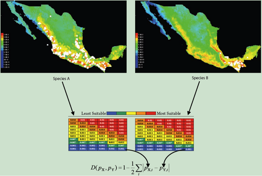
Let’s say we’ve got some observation based on real data.  In our case, we’ll say it’s a measurement of niche overlap between ENMs built from real occurrence points for a pair of species (figure partially  adapted (okay, stolen) from a figure by Rich Glor).  We have ENMs for two species, and going grid cell by grid cell, we sum up the differences between those ENMs to calculate a summary statistic measuring overlap, in this case D.
Picture
Due to some evolutionary or ecological question we’re trying to answer, we’d like to know whether this overlap is what we’d expect under some null hypothesis.  For the sake of example, we’ll talk about the “niche identity” test of Warren et al. 2008.  In this case, we are asking whether the occurrence points from two species are effectively drawn from the same distribution of environmental variables.  If that is the case, then whatever overlap we see between our real species should be statistically indistinguishable from the overlap we would see under that null hypothesis.  But how do we test that idea quantitatively?

In the case of good old parametric statistics, we would do that by comparing our empirical measurement to a parametric estimate of the overlap expected between two species (i.e., we would say "if the null hypothesis is true, we would expect an overlap of 0.5 with a standard deviation of .05", or something like that).  That would be fine if we could accurately make a parametric estimate of the expected distribution of overlaps under that null hypothesis, i.e., we need to be able to specify a mean and variance for expected overlap under that null hypothesis.  How do we do that?  Well, unfortunately, in our case we can’t.  For one thing we simply can’t state that null in a manner that makes it possible for us to put numbers on those expectations.  For another, standard parametric statistics mostly require the assumption that the distribution of expected measurements under the null hypothesis meets some criteria, the most frequent being that the distribution is normal.  In many cases we don’t know whether or not that’s true, but in the case of ENM overlaps we know it’s probably not true most of the time.  Overlap metrics are bound between 0 and 1, and if the null hypothesis generates expectations that are near one of those extremes, the distribution of expected overlaps is highly unlikely to be even approximately normal.  There can also be (and this is based on experience), multiple peaks in those null distributions, and a whole lot of skew and kurtosis as well.  So a specification of our null based on a normal distribution would be a poor description of our actual expectations under the null hypothesis, and as a result any statistical test based on parametric stats would be untrustworthy.  I have occasionally been asked whether it’s okay to do t-tests or other parametric tests on niche overlap statistics, and, for the reasons I’ve just listed, I feel that the answer has to be a resounding “no”.

So what’s the alternative?  Luckily, it’s actually quite easy.  It’s just a little less familiar to most people than parametric stats are, and requires us to think very precisely about the ideas we’re trying to test.  In our case, what we need to do is to find some way to estimate the distribution of overlaps expected between a pair of species using this landscape and these sample sizes if they were effectively drawn from the same distribution of environments.  What would that imply?  Well, if each of these sets of points were drawn from the same distribution, we should be able to generate overlap values similar to our empirical measurement by repeating that process.  So that’s exactly what we do!

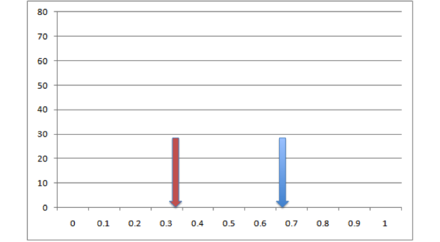
We take all of the points for these two species and we throw them in a big pool.  Then we randomly pull out points for two species from that pool, keeping the sample sizes consistent with our empirical data.  Then we build ENMs for those sets of points and measure overlaps between them.  That gives us a single estimate of expected overlaps under the null hypothesis.  So now we’ve got our empirical estimate (red) and one realization of the null hypothesis (blue)
Picture
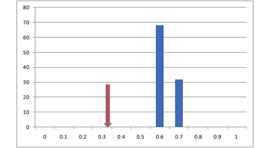
All right, so it looks like based on that one draw from the null distribution, our empirical overlap is a lot lower than you’d expect.  But how much confidence can we have in this conclusion can we have based on one single draw from the null distribution?  Not very much.  Let’s do it a bunch more times and make a histogram:
Picture
All right, now we see that, in 100 draws from that null distribution, we never once drew an overlap value that was as low as the actual value that we get from our empirical data.  This is pretty strong evidence that, whatever process generated our empirical data, it doesn’t look much like the process that generated that null distribution, and based on this evidence we can statistically reject that null hypothesis.  But how do we put a number on that?  Easy!  All we need to do is figure out what the percentile in that distribution is that corresponds to our empirical measurement.  In this case our empirical value is lower than the lowest number in our null distribution.  That being the case, we can’t specify exactly what the probability of getting our empirical result is, only that it’s lower than the lowest value we obtained, so it’s p < (whatever that number is).  Since we did 100 iterations of that null hypothesis (and since our empirical result is also a data point), the resolution of our null distribution is 1/(100 + 1) ~= .01.  Given our resolution, that means p is between 0 and .01 or, as we normally phrase it, p < .01.  If we’d done 500 simulation runs and our empirical value was still lower than our lowest value, it would be p < 1/(500 + 1), or p < .0002.  If we’d done 500 runs and found that our empirical value was between the lowest value and the second lowest value, we would know that .0002 < p < .0004, although typically we just report these things as p < .0004.  Basically the placement of our empirical value in the distribution of expected values from our null hypothesis is an estimate of the probability of getting that value if that hypothesis were true.  This is exactly how hypothesis testing works in parametric statistics, the only difference being that in our case we generated the null distribution from simulations rather than specifying it mathematically.

So there you go!  We now have a nonparametric test of our hypothesis.  All we had to do was (1) figure out precisely what our null hypothesis was, (2) devise a way to generate the expected statistics if that hypothesis were true, (3) generate a bunch of replicate realizations of that null hypothesis to get an expected distribution under that null, and (4) compare our empirical observations to that distribution.  Although this approach is certainly less easy than simply plugging your data into Excel and doing a t-test or whatnot, there are many strengths to the Monte Carlo approach. For instance, we can use this approach to test pretty much any hypothesis that we can simulate – as long as we can produce summary statistics from a simulation that are comparable to our empirical data, we can test the probability of observing our empirical data under the set of assumptions that went into that simulated data.  It also means we don’t have to make assumptions about the distributions that we’re trying to test – by generating those distributions directly and comparing our empirical results to those distributions, we manage to step around many of the assumptions that can be problematic for parametric statistics.

The chief difficulty in applying this method is in steps 2 and 3 above – we have to be able to explicitly state our null hypothesis, and we have to be able to generate the distribution of expected measurements under that null.  Honestly, though, I think this is actually one of the greatest strengths of Monte Carlo methods: while this process may be more intensive than sticking our data into some plug-and-chug stats package, it requires us to think very carefully about what precisely our null hypothesis means, and what it means to reject it.  It requires more work, but more importantly it requires a more thorough understanding of our own data and hypotheses.

The new R version of ENMTools is in the works! Here's how to build an enmtools.species object.

$
0
0
But for real this time.  I've started over entirely from scratch, and I'm using the new R package as a foundation for some novel analyses that I'm developing as part of my current research.  You can download it and view a fairly lengthy manual of what's currently implemented here:

https://github.com/danlwarren/ENMTools


For reasons that will become clear with time (when some of the downstream stuff gets finished), the way you interface with ENMTools is going to be a bit different from how you work with dismo or Biomod.  First off, you start by defining enmtools.species objects for each species (or population) that you want to compare.


Here I'll create one called ahli (based on data from Anolis ahli).


ahli = enmtools.species()

Now that doesn't have any data associated with it, so if we get a summary of it, we basically just hear back from R that we don't have any data.


ahli
## 
##
## Range raster not defined.
##
## Presence points not defined.
##
## Background points not defined.
##
## Species name not defined.

So let's add some data:


ahli$species.name = "ahli"
ahli$presence.points = read.csv("test/testdata/ahli.csv")[,3:4]

ahli$background.points = background.points.buffer(ahli$presence.points, 20000, 1000, env[[1]])


ahli


And then look at it again:


## 
##
## Range raster:
## class : RasterLayer
## dimensions : 418, 1535, 641630 (nrow, ncol, ncell)
## resolution : 0.008333333, 0.008333333 (x, y)
## extent : -86.90809, -74.11642, 19.80837, 23.2917 (xmin, xmax, ymin, ymax)
## coord. ref. : NA
## data source : in memory
## names : layer.1
## values : 1, 1 (min, max)
##
##
##
## Presence points (first ten only):
##
## | Longitude| Latitude|
## |---------:|--------:|
## | -80.0106| 21.8744|
## | -79.9086| 21.8095|
## | -79.8065| 21.7631|
## | -79.8251| 21.8095|
## | -79.8807| 21.8374|
## | -79.9550| 21.8374|
## | -80.3446| 22.0136|
## | -80.2983| 21.9951|
## | -80.1776| 21.9023|
## | -80.1591| 21.9673|
##
##
## Background points (first ten only):
##
## | Longitude| Latitude|
## |---------:|--------:|
## | -79.78726| 21.72920|
## | -79.82892| 21.73754|
## | -79.83726| 21.69587|
## | -80.01226| 22.01254|
## | -79.63726| 21.76254|
## | -79.92892| 21.78754|
## | -79.99559| 22.12920|
## | -79.81226| 21.87087|
## | -80.30392| 22.07920|
## | -79.97892| 21.85420|
##
##
## Species name: ahli

Neat, huh?  Next up I'll show you how to build an ENM.


Using an enmtools.species object to build an ENM

$
0
0
Now that we've got our enmtools.species object and have assigned it presence and background data and a species name, we can use it to build models very simply!  For this functionality, ENMTools is basically just acting as a wrapper for dismo, using those functions to actually build models.  At present ENMTools only has interfaces for GLM, Maxent, Bioclim, and Domain, but that will change with time.

So let's use our enmtools.species object "ahli" to build a quick Bioclim model.  I've got a RasterStack object made up of four environmental layers.  It's named "env", and the layers are just "layer.1", etc.

Let's build a model!

ahli.bc = enmtools.bc(species = ahli, env = env)

For Bioclim, Domain, and Maxent, it's that easy!  ENMTools extracts the presence and background data from env using the data stored in the species object, builds a model, and returns some lovely formatted output.

For GLM we need to supply a formula as well, but other than that it's idential.


ahli.glm = enmtools.glm(f = pres ~ layer.1 + layer.2 + layer.3 + layer.4, species = ahli, env = env)

Let's look at the output:

ahli.glm
## 
##
## Formula: presence ~ layer.1 + layer.2 + layer.3 + layer.4
##

##
##
## Data table (top ten lines):
##
## | layer.1| layer.2| layer.3| layer.4| presence|
## |-------:|-------:|-------:|-------:|--------:|
## | 2765| 1235| 1174| 252| 1|
## | 2289| 1732| 957| 231| 1|
## | 2158| 1870| 983| 253| 1|
## | 2207| 1877| 967| 259| 1|
## | 2244| 1828| 945| 249| 1|
## | 2250| 1766| 919| 235| 1|
## | 2201| 1822| 978| 277| 1|
## | 2214| 1786| 986| 284| 1|
## | 2287| 1722| 992| 266| 1|
## | 2984| 965| 1311| 237| 1|
##
##
## Model:
## Call:
## glm(formula = f, family = "binomial", data = analysis.df)
##
## Deviance Residuals:
## Min 1Q Median 3Q Max
## -0.67171 -0.20485 -0.14150 -0.09528 3.08762
##
## Coefficients:
## Estimate Std. Error z value Pr(>|z|)
## (Intercept) 46.178922 24.777923 1.864 0.0624 .
## layer.1 -0.013347 0.006276 -2.127 0.0334 *
## layer.2 -0.011985 0.006612 -1.813 0.0699 .
## layer.3 0.003485 0.006586 0.529 0.5967
## layer.4 -0.009092 0.021248 -0.428 0.6687
## ---
## Signif. codes: 0 '***' 0.001 '**' 0.01 '*' 0.05 '.' 0.1 '' 1
##
## (Dispersion parameter for binomial family taken to be 1)
##
## Null deviance: 164.58 on 1015 degrees of freedom
## Residual deviance: 150.15 on 1011 degrees of freedom
## AIC: 160.15
##
## Number of Fisher Scoring iterations: 8
##
##
##
## Suitability:
## class : RasterLayer
## dimensions : 418, 1535, 641630 (nrow, ncol, ncell)
## resolution : 0.008333333, 0.008333333 (x, y)
## extent : -86.90809, -74.11642, 19.80837, 23.2917 (xmin, xmax, ymin, ymax)
## coord. ref. : NA
## data source : in memory
## names : layer
## values : 6.419793e-08, 0.999983 (min, max)

plot of chunk unnamed-chunk-8
You get pretty, formatted output and a nice plot as well.  Next up: identity/equivalency tests!


Running an identity/equivalency test in the ENMTools R package

$
0
0
Okay, let's say we've got two enmtools.species objects: ahli and allogus.  How can we run an identity test?

Here's what we need:


  1. Our two species
  2. Our RasterStack of environmental layers
  3. The type of model we'd like ("glm", "bc", "dm", or "mx", for GLM, Bioclim, Domain, or Maxent)
  4. A formula (GLM only)
  5. The number of reps to perform

So here's how we'd run an identity test using GLM for our two species. 


id.glm = identity.test(species.1 = ahli, species.2 = allogus, env = env, type = "glm", f = presence ~ layer.1 + layer.2 + layer.3 + layer.4, nreps = 99)

Doing 99 reps takes a while, but when you're done, you get an "identity.test" object.  That contains all sorts of useful information.  A quick summary will show you some of it:

id.glm
## 
##
##
##
## Identity test ahli vs. allogus
##
## Identity test p-values:
## D I rank.cor
## 0.01 0.01 0.01
##
##
## Replicates:
##
##
## | | D| I| rank.cor|
## |:---------|---------:|---------:|----------:|
## |empirical | 0.2221752| 0.4661581| -0.4761597|
## |rep 1 | 0.8883545| 0.9899271| 0.8942366|
## |rep 2 | 0.8486324| 0.9828760| 0.9315827|
## |rep 3 | 0.8227838| 0.9742077| 0.8881490|
## |rep 4 | 0.7255044| 0.9469161| 0.5551645|
plot of chunk unnamed-chunk-14
If you want to access the empirical or replicate models, those are stored in that object as well:

names(id.glm)
[1] "description""reps.overlap""p.values""empirical.species.1.model""empirical.species.2.model"
[6] "replicate.models""d.plot""i.plot""cor.plot"

As with building species models, identity.test works pretty much the same for Domain, Bioclim, and Maxent models with the exception that you don't need to supply a formula.

Background/similarity tests in the ENMTools R package

$
0
0
Okay, let's use our two species to run a background/similarity test.  This works a lot like the identity test (see the post preceding this one), but there's a new option called "test.type" that can be set to "asymmetric" or "symmetric".  Here's an asymmetric background test using Bioclim:


bg.bc.asym = background.test(species.1 = ahli, species.2 = allogus, env = env, type = "bc", nreps = 99, test.type = "asymmetric")
bg.bc.asym
## 
##
##
##
## Asymmetric background test ahli vs. allogus background
##
## background test p-values:
## D I rank.cor
## 0.32 0.76 0.43
##
##
## Replicates:
##
##
## | | D| I| rank.cor|
## |:---------|---------:|---------:|---------:|
## |empirical | 0.1328502| 0.3177390| 0.0706201|
## |rep 1 | 0.1430965| 0.3114858| 0.0824412|
## |rep 2 | 0.1284871| 0.2801639| 0.0156034|
## |rep 3 | 0.1599120| 0.3384525| 0.1136082|
## |rep 4 | 0.1431022| 0.3101197| 0.0766638|
plot of chunk unnamed-chunk-17


What is "symmetric" vs. "asymmetric"?  Well, an asymmetric test means that we are comparing the empirical overlap to a null distribution generated by comparing one species' real occurrences to the background of another (species.1 vs. background of species.2).  In the Warren et al. 2008 paper we used this sort of asymmetric test, repeating it in each direction (species.1 vs. background of species.2 and species.2 vs. background of species.1).  While we had the idea that that might generate some interesting biological insight, I think it's generated just as much (if not more) confusion.  For this reason, the new R package also provides the option to do symmetric tests.  These tests compare the empirical overlap to the overlap expected when points are drawn randomly from the background of both species (species.1 background vs. species.2 background), keeping sample sizes for each species constant, of course.

And now a symmetric background test using Domain:


bg.dm.sym = background.test(species.1 = ahli, species.2 = allogus, env = env, type = "dm", nreps = 99, test.type = "symmetric")

bg.dm.sym
## 
##
##
##
## Symmetric background test ahli background vs. allogus background
##
## background test p-values:
## D I rank.cor
## 0.38 0.36 0.21
##
##
## Replicates:
##
##
## | | D| I| rank.cor|
## |:---------|---------:|---------:|---------:|
## |empirical | 0.1328502| 0.3177390| 0.0706201|
## |rep 1 | 0.2382775| 0.4428653| 0.1774936|
## |rep 2 | 0.1518903| 0.3555431| 0.1002003|
## |rep 3 | 0.1250674| 0.3029139| 0.0717565|
## |rep 4 | 0.1165355| 0.2946842| 0.0841041|
plot of chunk unnamed-chunk-20


New features for ENMTools model objects and functions: response plots, model evaluation, and new color ramps

$
0
0
One of the advantages of the enmtools.species object structure is that I can now provide a much more accessible interface to much of dismo's modeling functionality, and can add new functionality that automates a lot of the outputs you might typically want from an SDM/ENM.  You've already seen some of this here, but in the past week I've added a lot more.  For one thing I've switched from the default color ramps, such as this:


To viridis color ramps, e.g.,


This has a number of advantages.  First, viridis color ramps are very pretty, and this particular one has a very familiar Maxent-y sort of look about it which makes it easy for an experienced SDM modeler to interpret.  More importantly, the viridis color ramps are designed with accessibility in mind.  The authors put a ton of work into figuring out a set of color ramps that are interpretable when printed in greyscale AND accessible to people with varying types of color blindness.  That's pretty awesome.

You'll also notice that there are two sets of points plotted there.  Those are training and test points.  You can now call all of the enmtools modeling functions with an argument "test.prop", e.g.,

ahli.glm = enmtools.glm(pres ~ layer.1 + layer.2 + layer.3 + layer.4, ahli, env, test.prop = 0.2)

And they will automatically withhold that proportion of your data for model testing.  Now when you call your model object, you get training and test evaluation metrics!

>ahli.glm


Formula:  presence ~ layer.1 + layer.2 + layer.3 + layer.4


Data table (top ten lines): 

|   | Longitude| Latitude| layer.1| layer.2| layer.3| layer.4| presence|
|:--|---------:|--------:|-------:|-------:|-------:|-------:|--------:|
|1  |  -80.0106|  21.8744|    2765|    1235|    1174|     252|        1|
|2  |  -79.9086|  21.8095|    2289|    1732|     957|     231|        1|
|3  |  -79.8065|  21.7631|    2158|    1870|     983|     253|        1|
|4  |  -79.8251|  21.8095|    2207|    1877|     967|     259|        1|
|5  |  -79.8807|  21.8374|    2244|    1828|     945|     249|        1|
|6  |  -79.9550|  21.8374|    2250|    1766|     919|     235|        1|
|7  |  -80.3446|  22.0136|    2201|    1822|     978|     277|        1|
|8  |  -80.2983|  21.9951|    2214|    1786|     986|     284|        1|
|10 |  -80.1591|  21.9673|    2984|     965|    1311|     237|        1|
|11 |  -80.1498|  21.9858|    3042|     841|    1371|     221|        1|


Model:  
Call:
glm(formula = f, family = "binomial", data = analysis.df[, -c(1, 
    2)])

Deviance Residuals: 
     Min        1Q    Median        3Q       Max  
-0.65556  -0.18280  -0.12121  -0.08065   3.10812  

Coefficients:
             Estimate Std. Error z value Pr(>|z|)  
(Intercept) 40.033648  27.208173   1.471   0.1412  
layer.1     -0.012770   0.007165  -1.782   0.0747 .
layer.2     -0.009662   0.007346  -1.315   0.1884  
layer.3      0.006954   0.006638   1.047   0.2949  
layer.4     -0.020317   0.025631  -0.793   0.4280  
---
Signif. codes:  0 ‘***’ 0.001 ‘**’ 0.01 ‘*’ 0.05 ‘.’ 0.1 ‘ ’ 1

(Dispersion parameter for binomial family taken to be 1)

    Null deviance: 130.29  on 1011  degrees of freedom
Residual deviance: 119.18  on 1007  degrees of freedom
AIC: 129.18

Number of Fisher Scoring iterations: 8


Model fit (training data):  class          : ModelEvaluation 
n presences    : 12 
n absences     : 1000 
AUC            : 0.7485833 
cor            : 0.09753628 
max TPR+TNR at : -4.82228 


Proportion of data wittheld for model fitting:  0.2

Model fit (test data):  class          : ModelEvaluation 
n presences    : 4 
n absences     : 1000 
AUC            : 0.74075 
cor            : 0.05048264 
max TPR+TNR at : -4.570937 


So that's cool, obviously.  Even cooler is that your model object now contains marginal response functions.  These are calculated by varying each predictor from the minimum value to the maximum value found in the environmental layers, while holding the other predictors constant at the mean value across all presence points.  At present these plots aren't printed by default when you call your object, but I may change that.  For now, you can type:

>ahli.glm$response.plots

And you get:


I may do some more tweaking in the future, but these are ggplot2 plots so you can easily modify them however you want.

ENMTools R package model plots are now all done in ggplot2

$
0
0
Newest update (I did say they'd be coming very rapidly now, didn't I?): I've switched the enmtools model plots from using base raster plotting functions to using ggplot2.  They don't actually look very different, as you can see by comparing base (top) to ggplot2 (bottom) plots:


However the switch to ggplot2 allows for a lot more flexibility down the line, and also makes it easier to store plots as objects for future manipulation.

All rangebreak tests now available in ENMTools R package

$
0
0
As of yesterday, all rangebreak tests are now available in the R package.  There are still some rough edges to be smoothed off and all that, but if you are doing a rangebreak-y study and need that sort of thing, it is usable.  Demo code and example outputs are now available on the readme at:

https://github.com/danlwarren/ENMTools


Hey, what's up with those environmental overlaps in the ENMTools R package?

$
0
0
I'm so glad I asked!  The env.overlap metrics produced by the ENMTools R package are based on methods developed by John Baumgartner and myself.  The purpose of these metrics is to address one of the key issues with the niche overlap metrics currently implemented in ENMTools and elsewhere; the difference between the geographic distribution of suitability and the distribution of suitability in environment space.

Existing methods in ENMTools and most other packages measure similarity between models via some metric that quantifies the similarity in predicted suitability of habitat in geographic space.  While this may be exactly the sort of thing you'd like to measure if you're wondering about the potential for species to occupy the same habitat in an existing landscape, it can be somewhat misleading if the availability of habitat types on the landscape is strongly biased.  For instance, what if two species have very little niche overlap in environment space, but that overlap happens to occur in a combination of environments that turns out to be very common in the current landscape?

To illustrate, let's take two species (red and blue) and look at their niches in environment space:


So they're pretty different, right? But what if the only available environments in the study region occur in that area of overlap?  E.g., what if the current environment space is represented by the green area here?


Well then the only environments we have within which we can measure similarity between species happen to be those environments that are suitable for both!  This means that our measure of overlap between models in geographic space could be arbitrarily disconnected from the actual similarity between those models in environment space.  Depending on the sort of question we're trying to ask, that could be quite misleading.

The method of measuring overlap developed by Broennimann et al. (2012) deals with this issue to some extent.  However, those methods only work in two dimensions, and only work by using a kernel density approach based on occurrence points in environment space.  My guess is that that's still way better than what the original ENMTools approach did for most purposes, but it's not very useful if (for instance) you want to ask how similar the environmental predictions of a GLM are to, say, an RF model.  You simply can't do it.  Or if you want to ask questions in a higher dimensional space, you're basically out of luck.

So what can we do?  Can we figure out a way to measure overlap between two arbitrary models in a n-dimensional space?  It turns out that this is not easy to do exactly, but you can get approximate measures to an arbitrary level of precision fairly easily!

Our approach leverages the fact that R already has great packages for doing Latin hypercube sampling.  This allows us to draw random, but largely independent, points from that n-dimensional environment space.  We can then use dismo's predict function to project our models to those points in environment space, and measure suitability differences between species.  Obviously throwing just a couple of points into a 19-dimensional space (for instance, if you're using all Bioclim variables) isn't going to get you very close to the truth, but of course if you keep throwing more points in there you will get closer and closer to the true average similarity between models across the space.

SO that's what the method does: it starts by making a random Latin hypercube sample of 10,000 points from the space of all combinations of environments, with each variable bound by it's maximum and minimum in the current environment space.  Then it chucks another 10,000 points in there, and it asks how different the answer with 20,000 points is compared to the answer with 10,000.  Then repeat for 30,000 vs. 20,000, and so on, until subsequent measures fall below some threshold tolerance level.  This allows us to get arbitrarily close to the true overlap by specifying our tolerance level.  Lower tolerances take longer and longer to process, since it requires more samples for the value to converge.  However, we've found that with tolerances set at around .001 we get very consistent results for a 4-dimensional comparison with an execution time of around two seconds.

Pretty cool, huh?  Now you can compare the environmental predictions of any two models that can be projected using ENMTools' predict() function in environment space, instead of just looking at their projections into a given geographic space!

R users: update your R!

$
0
0
Hey y'all, if you're doing a bunch of SDM/ENM stuff in R and are finding that many of your operations are running really slowly, you should check your R version.  R version 3.3.0 has some sort of bug going on that causes it to handle many raster operations VERY slowly, including extracting data from a raster using points.

It's a very odd bug, because it causes the operation to get slower and slower the more points you add (which makes sense), but then suddenly gets considerably faster when you're using over 250 points.  So extracting data using 250 points might take three minutes, while 251 points takes three seconds.  Crazy, but at least the fix is easy!
Viewing all 100 articles
Browse latest View live